Citizen Data Scientist, Module III: Measuring Model Performance: Metrics That Matter
After building a machine learning model, the next crucial step is to evaluate how well it performs. In this module, we explore various metrics for assessing the performance of both regression and classification models. From understanding variance and error metrics to working with confusion matrices, precision, recall, and ROC curves, this post walks through the most important tools and concepts for measuring model performance.
Why Measuring Model Performance Is Essential
Once we have trained a model, how do we know if it’s any good? This is where performance metrics come into play. Metrics help us quantify how close our predictions are to the actual outcomes. For regression models, we want to measure how well the predicted values fit the true continuous values, while in classification tasks, we want to know how accurate the model is in assigning data points to discrete categories.

Regression Performance Metrics
For regression models, the goal is to predict continuous outputs, such as house prices or car mileage. Several metrics help us evaluate how well the model performs:

Example: Intuitive Understanding of R²
Imagine we’re predicting house prices based on features like size, location, and number of rooms. If the R² of our model is 0.85, that means 85% of the variability in house prices can be explained by the model. An R² of 0 would mean the model is no better than predicting the average price every time. A negative R² would mean our model is doing worse than even that baseline, possibly due to overfitting or poor feature selection
Classification Performance Metrics
Classification models, used to categorize data points (e.g., spam detection, medical diagnosis), require different metrics. The most common ones include:
Accuracy
Accuracy is the simplest and most intuitive metric, representing the percentage of correct predictions:

However, accuracy can be misleading, especially when the classes are imbalanced. For example, in a dataset with 90% "not spam" emails, a model that always predicts "not spam" will have high accuracy but will fail to catch actual spam emails.
Confusion Matrix
A confusion matrix gives a more detailed view of classification performance by counting:
True Positives (TP): Correctly predicted positive cases.
True Negatives (TN): Correctly predicted negative cases.
False Positives (FP): Incorrectly predicted positive cases.
False Negatives (FN): Incorrectly predicted negative cases.
This table provides the foundation for other key metrics like precision and recall
Precision, Recall, and F1-Score


When Recall Matters More Than Precision
Imagine you're developing a model to detect a rare but dangerous machine failure in an industrial setting. If the failure occurs, it could cause millions of dollars in damage. In this case, recall is crucial because missing even one failure (false negative) could be catastrophic. The model should flag every possible failure case, even if that means some false positives (incorrect alarms). False alarms can be handled, but missing a critical failure is much worse.
Conversely, in tasks where false positives are costly or problematic (e.g., spam filters where marking legitimate emails as spam is highly undesirable), precision would take priority.
Micro vs. Macro F1 Scores
When working with multiple classes, we calculate the F1-score for each class. The micro F1-score averages the individual class scores based on the number of samples, whereas the macro F1-score gives equal weight to all classes, regardless of size
ROC and AUC
The Receiver Operating Characteristic (ROC) curve plots the true positive rate (TPR) against the false positive rate (FPR) as we vary the decision threshold. A perfect classifier would achieve an area under the ROC curve (AUC) of 1, while random guessing yields an AUC of 0.5.
Example: Using ROC in Medical Diagnostics
In medical diagnostics, we can use ROC curves to evaluate models that predict whether a patient has a disease. A model with a high AUC (close to 1) means it’s good at distinguishing between patients with and without the disease. If the AUC is close to 0.5, the model is no better than random guessing
Variance and Bias in Model Performance
When evaluating models, two common problems can arise:
Overfitting: The model performs well on the training data but poorly on new data. This is often a result of high variance, where the model captures noise in the training data.
Underfitting: The model fails to capture the underlying trend in the data, typically due to high bias. It performs poorly on both training and test data
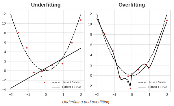
Overfitting in Predictive Maintenance
Imagine building a predictive maintenance model that uses thousands of sensor data points from machines. If the model is overfitting, it might perfectly predict when certain machines need maintenance in the training set but fail to generalize to new machines with slightly different behaviors. As a result, the model would have high variance and may perform poorly in real-world applications
K-Fold Cross-Validation
To avoid overfitting and better evaluate model performance, we can use k-fold cross-validation. Here’s how it works:
Split the data into k equal parts.
Train the model on k−1k-1k−1 parts and test it on the remaining part.
Repeat this process kkk times, each time using a different part as the test set.
Average the results across all folds to get a more reliable estimate of the model’s performance.
Conclusion: Metrics for Better Models
Understanding the strengths and weaknesses of different performance metrics is essential for building reliable models. Whether it’s regression or classification, knowing how to evaluate your model’s predictions ensures that it performs well on real-world data. By incorporating techniques like cross-validation, we can mitigate issues like overfitting and make informed decisions about model improvements.